Exploring Pathfinding Algorithms

Why Pathfinding?

The project was born from a curiosity to see how different search algorithms would solve the same maze. And why a maze? Well, it is intuitive for us to solve a maze starting from the end. I wanted to see how the algorithms would solve it beginning from the start of the maze as well as to see how they would fare against each other.

To put to the test, I used: Depth-First Search (DFS), Breadth-First Search (BFS), and A* algorithm.

Creating the Maze

Before I could test pathfinding algorithms, I needed a maze to navigate. So, I had to start by creating the maze first. I chose to generate maze using a recursive backtracking algorithm, which is essentially a depth-first search applied to maze construction. Although, it seems like this could bias the results, but if the maze generation starts randomly, while search starts systematically, this should be a valid test.

The core idea is simple: start with a grid where every cell has walls on all four sides. Pick a starting cell, mark it as visited, and then randomly choose an unvisited neighbor. Break down the wall between them, move to that neighbor, and repeat. When you hit a dead end (no unvisited neighbors), backtrack to the previous cell and continue from there.

Here's the key part of my implementation:

def maze_builder(self,ix,iy,count):
    start_cell = self.cell_at(ix,iy)
    valid_neighbours = self.nearest_neighbours(start_cell)
    if valid_neighbours==[]:
        self.done.append((ix,iy))
        if len(self.visited)>0:
            ix,iy = self.visited[-1]
            self.visited = self.visited[:-1]
    else:
        next_direction, next_cell = random.choice(valid_neighbours)
        start_cell.break_wall(next_cell,next_direction)
        self.visited.append((ix,iy))
        ix,iy = next_cell.x,next_cell.y
        count += 1
    return start_cell, ix,iy,count

The algorithm maintains a stack of visited cells. When there are no valid neighbors, we pop from the stack to backtrack. This guarantees that every cell will eventually be visited, creating a perfect maze where exactly one path exists between any two points. The image below shows a 15x15 maze generated by the algorithm. There is also an accompanying animation of the maze generation process.

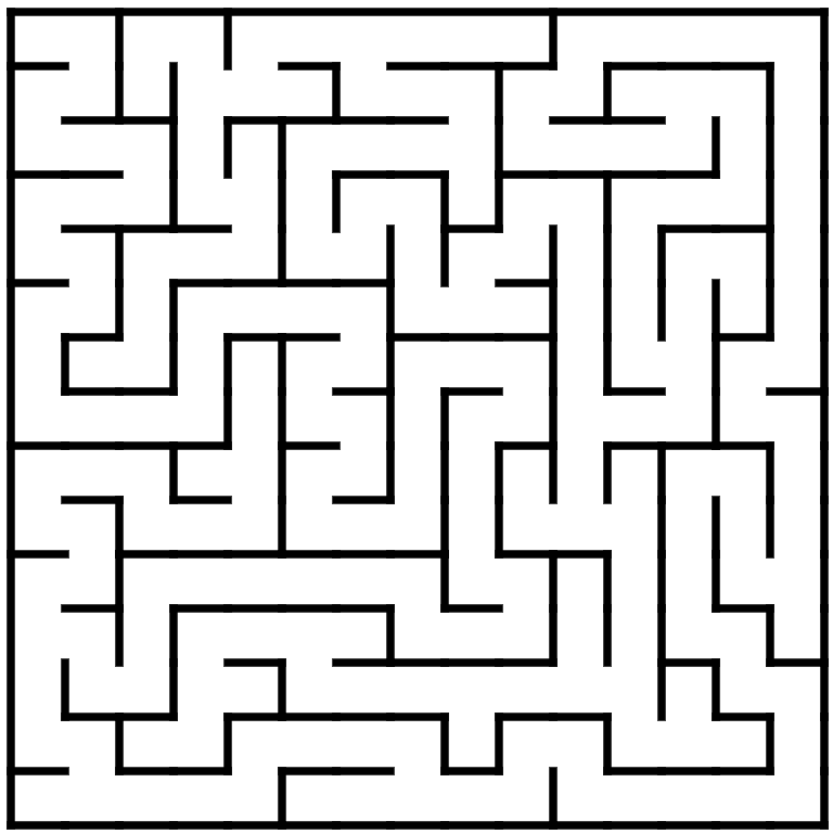
15x15 generated maze

Maze generation animation

Depth-First Search

DFS is the simplest conceptually. It explores as far as possible along each branch before backtracking. In maze terms, it picks a direction and keeps going until it hits a dead end, then backtracks.

def run(self,maze,ix,iy):
    cell = maze.cell_at(ix,iy)
    valid_neighbours = self.nearest_neighbours(cell,maze)
    if valid_neighbours==[]:

        self.done.append((ix,iy))
        if len(self.visited)>0:
            ix,iy = self.visited.pop(-1)
    else:
        next_cell = valid_neighbours[-1]
        self.visited.append((ix,iy))
        ix,iy = next_cell.x,next_cell.y
    return cell,ix,iy

DFS uses a LIFO stack , which I implement by popping from the end of the visited list. The visualization shows DFS taking long, winding paths, often exploring deep into dead ends before backtracking. It's not optimal for finding shortest paths, but it's memory-efficient and guaranteed to find a solution if one exists.

Breadth-First Search

BFS explores all neighbors at the current depth before moving to the next level. It's like a ripple expanding outward from the start point.

def run(self,maze,ix,iy):
    if (ix,iy) not in self.visited:
        self.visited.append((ix,iy))
    cell = maze.cell_at(ix,iy)
    valid_neighbours = self.nearest_neighbours(cell,maze)
    self.queue = self.queue + valid_neighbours
    for cells in valid_neighbours:
        self.visited.append((cells.x,cells.y))
    if valid_neighbours==[]:
        self.done.append((ix,iy))
    
    next_cell = self.queue.pop(0)
    ix,iy = next_cell.x,next_cell.y
    return cell,ix,iy

BFS uses a queue, implemented by popping from the front. Each cell tracks its parent, which allows us to reconstruct the path once we reach the goal. The visualization shows BFS expanding uniformly in all directions, like a wave. This guarantees the shortest path in an unweighted graph (which our maze is), but it explores many more cells than necessary.

A* Algorithm

While DFS and BFS seem too rigid in their implementation, A* tries to use a heuristic to make a more educated guess. So, instead of blindly exploring, the heuristic provides a compass that always points toward the destination. I used Manhattan distance for the heuristic because it's the most intuitive for a maze environment and it's easy. Just abs(x_diff) + abs(y_diff). No fancy math needed.

The algorithm uses the formula: f(n) = g(n) + h(n), where

• g(n) is the actual cost from the start to node n
• h(n) is the heuristic estimate from node n to the goal
• f(n) is the total estimated cost

def insertCell(self,cell):
    sum = cell.G + cell.H
    n = len(self.queue)
    if n == 0:
        self.queue.append(cell)
    elif sum > self.queue[-1].G+self.queue[-1].H:
        self.queue.append(cell)
    else:
        for i in range(n):
            if sum < self.queue[i].G+self.queue[i].H:
                self.queue.insert(i,cell)
                break
            elif sum == self.queue[i].G+self.queue[i].H:
                if cell.H < self.queue[i].H:
                    self.queue.insert(i,cell)
                else:
                    self.queue.insert(i+1,cell)
                break

A* finds the shortest path and explores fewer cells than BFS when the heuristic is admissible (never overestimates the true cost). Manhattan distance is admissible for grid-based mazes where you can only move in four directions. The visualization shows A* making a beeline toward the goal, exploring far fewer cells than BFS while still guaranteeing the optimal path.

More implementation details

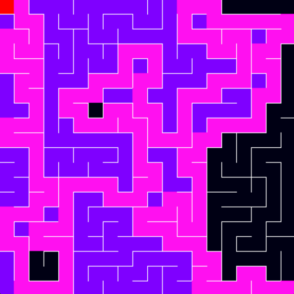
The visualization uses Pygame to render the maze and algorithm progress in real-time. Each algorithm step is drawn with a small delay (20ms), creating an animation effect. The current cell being explored is shown in red, visited cells in purple, and the final path in pink.

One challenge was handling the backtracking visualization. For BFS and A*, I track parent pointers and reconstruct the path once the goal is reached. For DFS, I simply reverse the visited list since DFS naturally explores a path from start to finish, though not necessarily the optimal one.

My Learnings from the project

I learned some key concepts. DFS uses a stack, BFS uses a queue, and A* uses a priority queue. The choice fundamentally changes the exploration pattern. DFS is memory-efficient but not optimal. BFS is optimal but explores many unnecessary cells. A* is optimal and efficient but requires a good heuristic. The code is straightforward Python, but the algorithms themselves are elegant solutions to a fundamental problem in computer science.

Also, watching the algorithms run makes their differences immediately apparent in a way that code alone doesn't convey. There's something deeply satisfying about watching a computer methodically solve a problem, especially when you understand exactly how it's thinking.

Alright folks, that's it for this project. See you in the next one!