Introduction
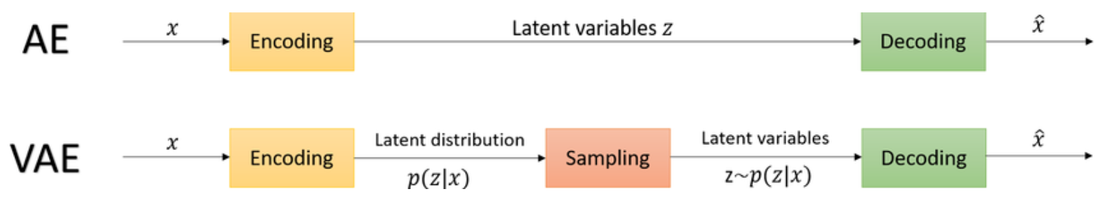
Having worked on diffusion models before, I wanted to understand what led to the inception of these models. The key foundation is the latent space which was introduced in the Variational Autoencoder model. VAEs themselves spun out of Autoencoders, which are a pair of encoder and decoder networks that learn to compress and then reconstruct the input data.
The compressed space can be thought of as a lower-dimensional hidden or latent space. The problem, however, is that the latent space in autoencoders is not "smooth" and forms disconnected clusters. This means that an image representation of an apple could be next to that of a horse, when it should be next to that of a cherry (both are round, red fruits). Autoencoder merely encodes in a smaller dimension, without caring about the semantic meaning of the data.
VAE tries to address this issue by forcing the latent space to be smooth and continuous, such that sampling from near horse images should yield zebra or donkey (or any other similar looking animal) images.
Problem Setup
Before diving into the code (or the math), I wanted to think about the problem setup.
The images reside in an input space. For MNIST, the images are of size 28x28 pixels, which is a 784 dimensional vector. Thus, in a 784 dimensional space, an image is a point. Further, most of the points in this space are noise, and only a small subset of the points are actual images. Now, suppose we wanted to generate a new image. We could model the input space with a neural network, and keep generating a 784 dimensional vector, which falls in the actual image space.
The problem, however, is that learning the small subset of digit images in an already small subset of actual images is difficult, since the input space is extremely high-dimensional, and hence sparse. So, the idea is to take this small subset, and represent it in a lower-dimensional space, such that the distance between the points in this space is meaningful.
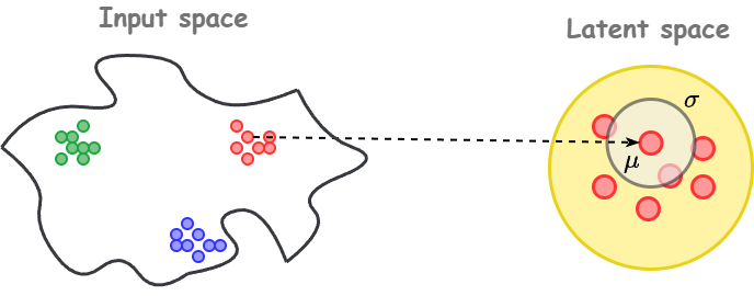
If we map the input image directly into the latent space, then we have a one to one mapping between the image and its latent. But this loses an important property: we want the representation to reflect not just the image itself, but also its similarity to nearby images.
Hence, we encode the image ($x$) into a mean ($\mu(x)$) and variance ($\sigma^2(x)$). The mean points to the cluster corresponding to that digit (e.g., all “3”s). The variance indicates how ambiguous or clear the image is, for instance, a messy “3” that looks like an “8” should have higher variance.
The mean and variance form a gaussian distribution, from which we sample a $z$. This $z$ is then sent to the decoder to get a reconstructed image. One component of our loss function would be to decrease the distance between the original image and the reconstructed image.
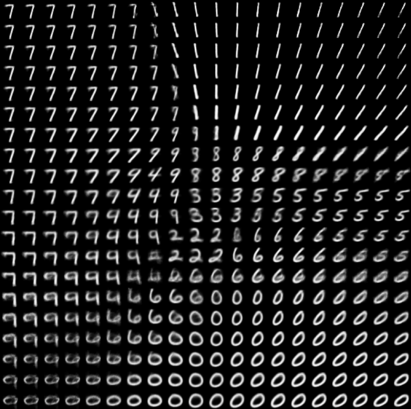
The other thing to consider is how will the latent space look. We want the latent space to be smooth and continuous, such that similar images are next to each other, and we can see a smooth transition when going form one image to the other. Since we need to enforce smoothness, we choose a simple function like a gaussian distribution for the latent space. This is the second loss term. We want to reduce the distance between the constructed and enforced latent space.
Math
Our aim is to learn the input distribution $p(x)$, for which we first learn the latent distribution $p(z)$. As mentioned above, $p(z) \sim \mathcal{N}(0,1)$. We also represent the encoding process as $p(z|x)$ and the decoding or generation process as $p(x|z)$. Now, $$p(z|x) = \frac{p(x,z)}{p(x)} = \frac{p(x,z)}{\int_{z} p(x|z).p(z)}$$ To compute the integral, we need to sum over the entire latent space, which is intractable. So, $p(z|x)$ cannot be calculated directly. One way to solve this is to approximate the generation function as $q_{phi}(z|x)$. We want this approximate function to be close to $p(z|x)$, and hence we want to reduce the KL divergence between them. $$min_{\phi} \; D_{KL} \;\left(q_{\phi}(z|x) \;\|\; p(z|x)\right)$$ Now, $D_{KL}(q(x) || p(x)) = \int_{x} q(x) \log \frac{q(x)}{p(x)}$. This gives us, $$\begin{align} D_{KL} \;\left(q_{\phi}(z|x) \;\|\; p(z|x)\right) &= \int_{z} q_{\phi}(z|x) \log \frac{q_{\phi}(z|x)}{p(z|x)}\\ &= \int_{z} q_{\phi}(z|x) \log \frac{q_{\phi}(z|x).p(x)}{p(x,z)}\\ &= \int_{z} q_{\phi}(z|x) \log \frac{q_{\phi}(z|x)}{p(x,z)} + \int_{z} q_{\phi}(z|x) \log p(x)\\ &= -\mathcal{L}(\phi) + \log p(x)\\ \end{align}$$ where, $$\mathcal{L}(\phi) = \int_{z} q_{\phi}(z|x) \log \frac{p(x,z)}{q_{\phi}(z|x)}$$ We can rearrange the terms to get, $$\mathcal{L}(\phi) = \log p(x) - D_{KL} \;\left(q_{\phi}(z|x) \;\|\; p(z|x)\right)$$ Now, KL-divergence is always non-negative, and hence, $$\mathcal{L}(\phi) \leq \log p(x)$$ $\mathcal{L}(\phi)$ is known as the evidence lower bound (ELBO). And minimizing the initial objective is equivalent to maximizing the ELBO. Maximizing ELBO also maximizes $p(x)$, which is the probability of the input data. This means we are assigning high probability to the observed $x$.
So, our new objective becomes maximizing the ELBO, which means we need to compute it's gradients. $\mathcal{L}_{\phi}$ depends not only on $\phi$, but also on $\theta$, where $$\begin{align} \mathcal{L}({\theta,\phi}) &= \int_{z} q_{\phi}(z|x) \log \frac{p_{\theta}(z|x).p(x)}{q_{\phi}(z|x)}\\ &= \mathbb{E}_{z \sim q_{\phi}(z|x)} \left[ \log \frac{p_{\theta}(z|x).p(x)}{q_{\phi}(z|x)} \right]\\ \end{align}$$ Assuming we have a set of $z^{(l)}$ sampled from $q_{\phi}(z|x)$, $l = 1,2,...,L$, we can approximate the above expression using Monte Carlo approximation as, $$\mathcal{L}({\theta,\phi}) \approx \frac{1}{L} \sum_{l=1}^{L} \log p_{\theta}(x,z^{(l)}) - \log q_{\phi}(z^{(l)}|x)$$ Fixing $z$, which is sampled, the gradient w.r.t. $\theta$ is straightforward, $$\nabla_{\theta} \mathcal{L}({\theta,\phi}) = \sum_{l=1}^{L} \nabla_{\theta}\log p_{\theta}(x,z)$$ However, we cannot directly take the gradient w.r.t. $\phi$, since $z$ is sample from $q_{\phi}(z|x)$. And sampling breaks the computation graph, since it is not differentiable.
To handle this, we use the reparameterization trick. Instead of sampling $z$ from $q_{\phi}(z|x)$, we get the $\mu$ and $\sigma$ of the gaussian distribution we want to create. We then recreate a gaussian using $\epsilon \sim \mathcal{N}(0,1)$, such that $$z = \mu_{\phi}(x) + \sigma_{\phi}(x) \cdot \epsilon$$ This ensures that gradients can flow through $\mu$ and $\sigma$. And hence, our ELBO becomes differentiable.
The ELBO can be simplified further as, $$\begin{align} \mathcal{L}({\theta,\phi}) &= \mathbb{E}_{z \sim q_{\phi}(z|x)} \left[ \log \frac{p_{\theta}(z|x).p(x)}{q_{\phi}(z|x)} \right]\\ &= \mathbb{E}_{z \sim q_{\phi}(z|x)} \left[ \log \frac{\log p(x)}{q_{\phi}(z|x)} \right] + \mathbb{E}_{z \sim q_{\phi}(z|x)} \left[ p_{\theta}(z|x) \right]\\ &= -D_{KL} \; \left(q_{\phi}(z|x) \;\|\; p(x) \right) + \mathbb{E}_{z \sim q_{\phi}(z|x)} \left[ \log p(z|x) \right]\\ \end{align}$$ The KL-divergence between 2 gaussians is given by, $$D_{KL} \; (q\|p)=\tfrac{1}{2}\left[\log\frac{|\Sigma_q|}{|\Sigma_p|}-d+\mathrm{Tr}(\Sigma_p^{-1}\Sigma_q)+(\mu_p-\mu_q)^\top\Sigma_p^{-1}(\mu_p-\mu_q)\right]$$ Plugging in the values, the ELBO simplifies to, $$\begin{align} \mathcal{L}({\theta,\phi}) \approx \tfrac{1}{2} \sum_{d=1}^{D} \left(1 + \log {\sigma_{\phi}^{2}}(x)_i - {{\mu_{\phi}}^2(x)_i} - {{\sigma_{\phi}}^2(x)_i} \right) + \frac{1}{L} \sum_{l=1}^{L} \log p_{\theta}(z^{(l)}|x)\\ \end{align}$$
Implementation
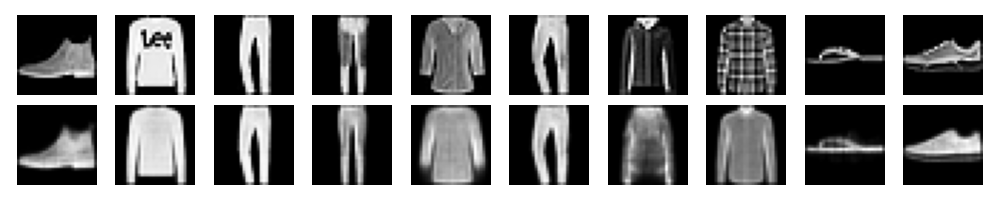
For the VAE, I used a 2 layer MLP for the encoder and decoder. I ran the model on MNIST and Fashion-MNIST datasets. Since the MNIST is not too complex, I used 20 dimensions for the latent space. The reconstructed images for Fashion-MNIST are shown below.